Power Spectrum Analysis using Spectral Estimators

 

The correlation of two time dependent functions g and h can be defined as follows:

If we denote the Fourier transform pairs by the symbol `` '' the Wiener-Khinchin Theorem states that the correlation of a function with itself (the auto-correlation) is related to its Fourier transform as follows:

where

and t and f are time and frequency respectively. Therefore, the absolute value of the Fourier transform of an ACF is the related power spectrum or power spectral density (PSD) function. Since we are dealing with sampled data over a finite period of time, we can obtain only an estimate of the spectrum. It is for this reason that various methods of PSD estimation are considered.

The SuperDARN radar measures the ACF of the scattered signal. Full spectral analysis of these ACFs goes beyond the simple phase analysis considered in section 3.5.1 and can resolve its shortcomings. On the other hand spectral analysis has its own difficulties and the methods used have to be carefully considered. Table 3.4 lists some of the possible methods for spectral analysis. The complexity of the algorithm for a given method is the number of computationally ``expensive'' operations such as multiplications or divisions.

  
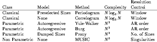
Table 3.4: Some Spectral Estimation Methods, after Marple (1987)

The classical methods typically employ the Fast-Fourier Transform (FFT) algorithm and are the most computationally efficient spectral estimation methods available. The PSD estimates are linearly proportional to the power of sinusoids present in the data. The main disadvantage is the distorting impact of sidelobe leakage due to inherent windowing of finite data. Window weighting of the data can reduce the effect of sidelobes at the expense of decreasing the spectral resolution. Statistical stability can be achieved by ensemble averaging, further reducing resolution. Generally, the resolution of the classical methods can be no better than the reciprocal of the total sampling time, independent of the characteristics of the data. The method is therefore not well suited for short data records. One should also note that using linear- or cubic-spline interpolation of data to increase resolution will increase sidelobes and decrease sensitivity at higher frequencies [Ach78]. Alternative methods, such as the parametric models, may improve or maintain high resolution without sacrificing much statistical stability. The transformation relationship between the ACF and the PSD by Fourier transformation is a non-parametric description of a second-order statistic. A parametric description may be devised by assuming a time series model of a random process. The PSD of such a model will then be dependent on the model parameters and not on the original ACF data.

The parametric approach to spectral estimation involves three steps: select a parametric time-series model to represent the measured data (autoregressive or AR, moving average or MA and combined autoregressive-moving average or ARMA), estimate the parameters of the model and finally insert the parameters into the theoretical PSD expression for that model. The characteristics of these methods are as follows.

• Parametric methods have a good frequency resolution even on small data sets; this is their main advantage.
• Spurious peaks are generated if a large model order is selected relative to the number of data samples, so model order selection is very important.
• The non-linear relationship of spectral power to actual power exhibited by most parametric methods makes absolute power measurements meaningless, so only relative power measurements are possible.

To illustrate the effect of various estimators, consider a spectrum with peaks at -0.15/ , 0.1/ , 0.2/ and 0.22/ and colored noise from -0.5/ to -0.2/ and from 0.2/ to 0.5/ , as shown in Figure 3.7 [Mar87, PFTV86]. Figure 3.8 shows a complex ACF of 64-lags length that has been analytically determined from this spectrum and PSD estimates derived by various methods from the ACF. The sample frequency is , where is the lag unit.

  
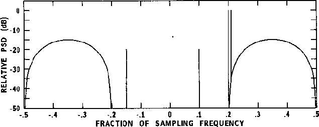
Figure 3.7: Analytically determined spectrum of test data process; after Marple (1987), page 17

  
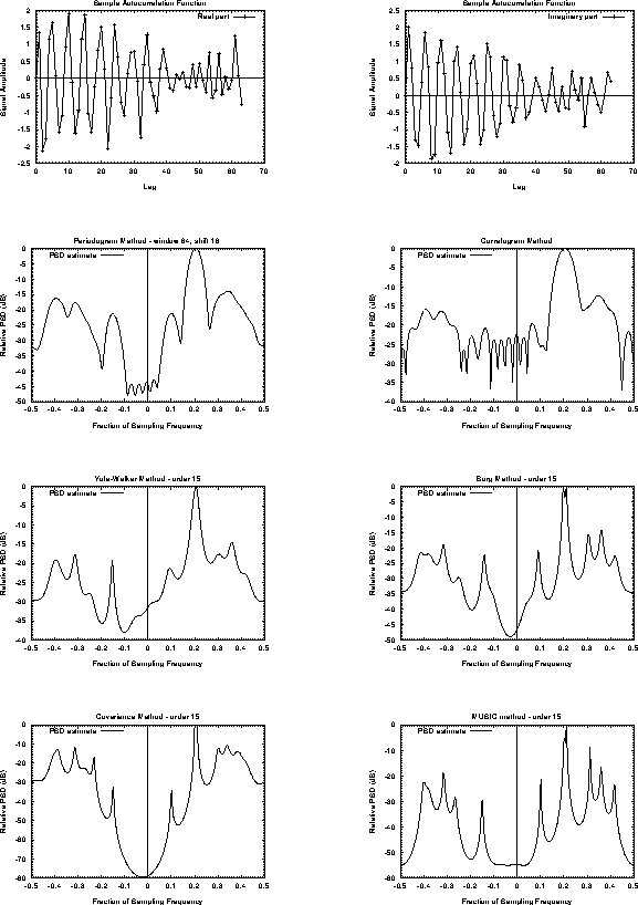
Figure 3.8: Comparison of the results from various spectral estimators for the test 64-lag complex autocorrelation function (first row)

Parametric models have been extensively used in the analysis of radar observations since they have been devised several decades ago. For example Haykin et. al [HCK82] describe the use of the maximum-entropy spectral estimator for the analysis of radar clutter as encountered in an air traffic control environment.