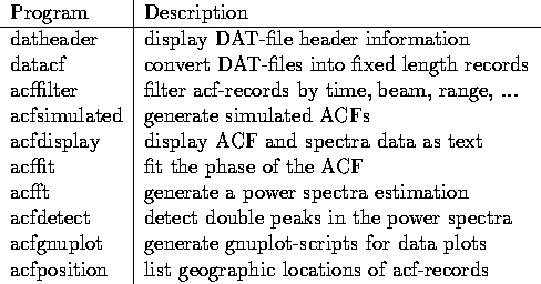
Table A.1: List of SuperDARN autocovariance function processing programs
Table A.1 lists a collection of programs which facilitate advanced processing of SuperDARN generated autocovariance function datasets that are stored in .DAT files.

Table A.1: List of SuperDARN autocovariance function processing programs
*** Program
        datheader
*** Usage
        datheader [DAT-file]
*** Synopsis
        Prints the information that is contained in the header of 'DAT-file'
        and the header of the first DAT record for informational purposes.
*** Example
        datheader test.dat


*** Program
        datacf
*** Usage
        datacf [DAT-file] >outfile
*** Synopsis
        Read in 'DAT-file' and convert the data into the fixed-length 'acf'
        records for use with other acf___ tool programs (see acf.h).
        The output is directed to 'stdout' for piping into another filter.
        The program will remove bad data points and interpolate linearly
        missing points in the ACF. Also some variables in the ACF-record
        will be calculated.
*** Example
        datacf test.dat >test.acf


*** Program
        acffilter
*** Usage
        acffilter [option] [option] ... <infile >outfile
        Options:
                h                 - this helptext
                n [Rec#-Range]    - define record-number range
                b [Beam-Range]    - define beam range
                r [Range-Range]   - define range range
                t [Time-Range]    - define time range
                s [SNR-Range]     - define a signal-to-noise limit,
                v                 - verbose processing, default: off
        Notes: Time-Range= 'YY MM DD HH MM SS' (enclose the numbers
        defining a time in quotes). Other ranges are two number
        separated by a space.
*** Synopsis
        This is the universal filter for acf-records. One can select record,
        beam, range, time and signal-to-noise ranges. Several filter options
        can be combined. Every filter option requires two numerical
        arguments defining an ascending range of values.
*** Example
        datacf test.dat | acffilter b 3 4 r 20 30 >filtered-test.acf


*** Program
        acfsimulated
*** Usage
        acfsimulated [Options] >outfile
        options:
                -h        this helptext
                -a#       number of ACF's to generate
                -n#       number of peaks in each spectrum (1-3)
                -g#       add a GS signal of amplitude # to spectrum
                -r        position first peak at random
                -R        vary number of Gaussian
                -N#       noise amplitude (0.0-1.0)
                -0# -9#   toggle missing lag at position #
*** Synopsis
        This routines creates artificial acf-records. It first generates
        random parameters of Doppler-velocity spectral peaks, generates
        the spectrum, optionally adds noise and simulates ACF's by
        Fourier-transforming the spectrum. The position of the first peak
        is varied as a function of record number. This can be overridden
        with the -r option. The total number of ACF's generated is
        controlled with the -a option and defaults to 1. The amplitudes
        should be in the range of 0.0 to 1.0. Up to 10 missing lags can
        be simulated with the -0, -1, -2, to -9 options.
*** Example
        acfsimulated -a5 -n2 -r -g0.8 -N0.1 | acfdisplay


*** Program
        acfdisplay
*** Usage
        acfdisplay <infile >outtext
*** Synopsis
        This program will simply read in acf-records and print out the ACF
        and spectral data as a text file in ASCII format. This feature is
        useful for debugging purposes.
*** Examples
        acfsimulated | acfdisplay
        acfsimulated -a10 | acfdisplay | more


*** Program
        acffit
*** Usage
        acffit <infile >outfile
*** Synopsis
        This program will attempt to find the mean phase of the ACF but
        using the 'brute=force' approach. The result will be stored in
        the first velocity entry of the acf-record.
*** Example
        Compare the output of the following command lines:
         acfsimulated -a10 -N0.2 | acfdisplay | grep "Center"
         acfsimulated -a10 -N0.2| acffit | acfdisplay | grep "Center"


*** Program
        acfft
*** Usage
        acfft [options] <infile >outfile
        Options:
                p <samples> <shift>     - Periodogram
                l <lags>                - Correlogram
                y <order>               - Yule-Walker
                b <order>               - Burg
                c <order>               - Covariance
                m <order>               - Modified Covariance
                a <order> <order> <lag> - ARMA
                v <order>               - Minimum Variance
                u <order> <signals>     - MUSIC
                e <order> <signals>     - EV
                S                       - Smooth output
                M                       - MEAN removal in real part of ACF
                N                       - Normalize maximum of psd to 1.0
*** Synopsis
        This routine performs a spectral estimation on the complex ACF and
        stores the spectrum in the acf-record. Several methods can be used
        - see the README file of the spectrum-library for details.
        The output can be smoothed (3 point average), the mean from the ACF
        can be removed before processing (to avoid groundscatter
        contamination in FFT based estimators) and the resulting spectrum
        can be normalized to a range from 0.0 to 1.0.
*** Example
        datacf test.dat | acffilter n 0 9 | acfft p 32 16 | acfdisplay


*** Program
        acfdetect
*** Usage
        acfdetect [options] <infile >outfile
        acfdetect v [options] <infile >outfile 2>logfile
        Options:
                c [value]   - set cutoff to [value], default=0.15
                m [value]   - set maximum peak sep. to [value] m/s
                z [value]   - set zero velocity range to [value] m/s
                v           - be verbose, default: off
*** Synopsis
        This routine will attempt to detect double-peaks in a power
        spectrum. The three step process involves: 1.) removing
        all signals below a certain cutoff level set by 'c'. 2.)
        Determining the number and location of all remaining local maxima.
        3.) Select all records with 2 peaks that are separated more than
        a value (set by 'z') from zero and are at the most some value (set
        by 'm') apart.
*** Example
        acfsimulated -a100 -n2 | acfdetect | acfdisplay | grep "#"


*** Program
        acfgnuplot
*** Usage
        acfgnuplot [options] <infile >gnuplot-script 2>logfile
        Options:
                p               - generate power spectrum plot
                a               - generate real/imaginary ACF plot
                l [label]       - label power spectrum curve with [label]
*** Synopsis
        This program will convert ACF and spectral data into a plotting
        script that can be executed directly by the 'gnuplot' program.
        It will generate one graph per page and stores the output in the
        file 'psd.ps'. For power spectrum generation use the 'p' option; for
        ACF generation use the 'a' option. Use the 'l' option to change the
        label pf spectra from 'PSD' to something else. On 'stderr', a single
        line containing location, time and page information for each graph
        will be printed. Captured into a logfile this should help identify
        particular events.
*** Example
        datacf test.dat | acfft b 8 | acfgnuplot | gnuplot


*** Program
        acfposition
*** Usage
        acfposition [options] <infile
        Options:
                a               read read beam/range pairs as ASCII
                v               be verbose, default: off
                r [value]       determines radar (1-12)
        Radars:
                1 = goose bay
                2 = schefferville
                3 = kapuskasing
                4 = halley
                5 = saskatoon
                6 = british columbia
                7 = alaska
                8 = stokkseyri (Iceland W)
                9 = iceland east
                10 = finland
                11 = sanae (durban)
                12 = syowa (Japan)
*** Synopsis
        This program will report the geographic position of the beam/range
        target regions of the radar. It will read the beam/range coordinates
        either from acf-records or if the 'a' option is selected from an
        ASCII file in a format that similar to the logfile of the 'acfdetect'
        program, i.e.
                text text [BEAM] text [RANGE]
        where BEAM and RANGE are the actual numbers. Ranges <5 are not
        considered. The latitude/longitude coordinates are degrees-north
        and degres-east.
*** Example
        acfsimulated -a10 | acfposition r 1